
By Jack Sun · Updated October 20, 2026
For a pleated metal cartridge, the most useful pressure-drop estimate comes from a clean flow–pressure-drop curve for the actual element and relevant fluid conditions. If the required flow lies between measured points, interpolate within that range. A validated model or a documented manufacturer coefficient can support other estimates, but cartridge length and a micron label alone cannot establish pressure drop.
This guide explains pleated filter pressure drop for industrial metal cartridges, particularly clean, single-phase liquid service. It explains how to read the curve and estimate pressure drop at a specified flow. Determining the actual system operating point requires additional system information. Gas flow, non-Newtonian liquids and two-phase service need their own validated data or model.
Which pressure difference is being calculated?
Pressure drop, Δp, is the upstream pressure minus the downstream pressure across defined measurement locations. Record those locations before comparing results. A curve for a filter medium, a complete cartridge and an installed housing can describe different losses.
| Quantity | What it describes | What it does not establish |
|---|---|---|
| Clean pressure drop | Flow resistance of the clean item under stated conditions | Its maximum permitted differential pressure. |
| Loaded pressure drop | Resistance after a defined contamination or service history | A universal cleaning interval or remaining life. |
| Allowable differential pressure | A design or validated operating limit for a stated assembly, temperature and direction | The clean flow resistance. |
| Housing working pressure | The housing’s applicable pressure limit | The element’s permitted differential pressure. |
A cartridge can operate in a high-pressure system while experiencing a much smaller pressure difference across its wall. Conversely, knowing the system pressure does not determine the element differential pressure. Keep normal flow, reverse flow and any transient conditions identified separately.
The information needed before using a curve
A curve is useful when its test object and conditions match the question. Begin with an identified cartridge: medium, grade or retention designation, layers, dimensions, pleat arrangement, core, supports, connections and flow direction. A nominal filtration rating does not identify all of those features.
| Information | What to record | Why it changes the interpretation |
|---|---|---|
| Fluid | Composition, temperature, viscosity and density where needed | Establishes the test conditions and whether corrections are justified. |
| Flow | Units and actual flow through the tested item | Separates one-element flow from the total system flow. |
| Element condition | Clean, previously used or cleaned; preparation history | Prevents different resistance states being combined. |
| Measurement | Pressure-tap boundaries, fixture and any housing correction | Shows which losses are included. |
| Data quality | Test date, instrument information, repeatability and usable range | Supports the confidence placed in an estimate. |
For hydraulic filters, ISO 3968:2017 addresses evaluation of differential pressure versus flow, including different viscosities and relevant assembly parts. Its scope is hydraulic filtration; referring to it does not establish that a particular cartridge has been tested to that standard. Agree the applicable method and required report for the project. [1]
How to read a flow–pressure-drop curve
Read the axes, legend and notes before taking a value from the line. A lower line is useful only when the compared curves describe relevant, comparable filters and conditions.
- Check the axes and units. Flow is often on the horizontal axis and differential pressure on the vertical axis, but some charts reverse them. Convert L/min, m³/h or gpm consistently; do the same for bar, kPa or psi.
- Identify the plotted item. Is the line for a medium, one complete cartridge, an empty housing or an installed assembly? Different lines may represent different media or constructions.
- Read the test conditions. Identify the fluid, temperature, viscosity, flow direction and element condition.
- Locate the requested flow. Move to the relevant curve, then read pressure drop on the other axis. On logarithmic axes, convert the plotted coordinates correctly; equal distances on the page do not mean equal numerical increments.
- Check the measured range. Do not treat the region beyond the endpoints as validated. Near a limit, request the original values and measurements close to the required flow.
The number of decimal places printed beside a curve does not establish measurement accuracy. Reading an image also introduces uncertainty from its resolution, line thickness and source.
Estimating pressure drop between measured values
When adjacent measurements bracket the requested flow, piecewise linear interpolation provides a transparent estimate. For points (Q₁, Δp₁) and (Q₂, Δp₂), use:
f = (Q − Q₁) / (Q₂ − Q₁)
Δp = Δp₁ + f × (Δp₂ − Δp₁)
Use matching flow units and matching pressure units. Q₂ must differ from Q₁, and Q must lie between them. The calculation connects two measurements with a straight segment; it does not prove that the underlying physical curve is straight.
Consider these invented numbers for a clean cartridge at one fixed liquid condition and measurement boundary:
| Flow, L/min | Pressure drop, kPa | Meaning |
|---|---|---|
| 20 | 12 | Illustrative lower point. |
| 40 | 28 | Illustrative upper point. |
| 30 | 20 | Interpolated point: f = (30 − 20)/(40 − 20) = 0.5. |
The result is 12 + 0.5 × (28 − 12) = 20 kPa. These numbers are an arithmetic example, not our product test data or a recommended operating condition. They also show why a line drawn from the origin through one point can give a different answer.
The measured filter flow and pressure-drop calculator accepts two to six measured pairs and queries between neighboring points. It requires comparable conditions and blocks extrapolation. It does not correct viscosity, infer permeability or assign a certified pressure rating. Use additional measurements where curvature matters, especially near an acceptance limit.
Adding cartridge and housing losses without counting them twice
Suppose the interpolated 20 kPa describes only the complete cartridge. At the same 30 L/min, assume another 5 kPa covers the housing and connections outside that cartridge boundary. For this simplified assembly:
Δp assembly = Δp cartridge + Δp remaining passages = 20 + 5 = 25 kPa
The additional 5 kPa is invented for this example. The terms must describe compatible conditions and boundaries that can be added without omissions or overlap. If the original curve already includes that housing, adding another 5 kPa counts it twice. Installation can also change the flow within a housing, so combining separately obtained component data needs an applicable, validated method. Parker’s DF25 documentation illustrates separate housing and element contributions for that specific product; its coefficients and limits are not assigned to Alloyfilter cartridges here. [6]
If four identical cartridges operate in parallel at a total flow of 120 L/min, a single-cartridge query at 30 L/min is justified only under an equal-flow assumption supported by the installation. The pressure drops of the four parallel cartridges are not added as 4 × 20 kPa. Assess common passages at their own flow and avoid adding overlapping losses. Different branch resistance or loading can invalidate an equal split.
Viscosity correction: where proportional estimates apply
For a fixed clean porous structure with predominantly viscous, laminar resistance and an approximately incompressible Newtonian liquid, a Darcy-type approximation makes the medium pressure drop proportional to dynamic viscosity and flow. ISO 4022:2018 distinguishes viscous and inertial permeability contributions for applicable permeable sintered metal test pieces; that distinction matters when deciding whether a simple proportional model is adequate. [2]
Under those restricted conditions, an estimate for the same identified structure is:
Δp₂ ≈ Δp₁ × (μ₂/μ₁) × (Q₂/Q₁)
Here μ is dynamic viscosity; the viscosity ratio must use the same units. The geometry and relevant permeability must remain unchanged. This relationship is not a general correction for an entire housing and cartridge when entrances, fittings, core flow or other inertial losses are significant.
For a separate illustrative calculation, suppose the identified medium’s viscous contribution is 12 kPa at 2 mPa·s. At the same flow and geometry, a viscosity of 3 mPa·s gives an estimate of 12 × 3/2 = 18 kPa for that contribution. This does not establish the new total assembly pressure drop, and it is not a correction of the earlier interpolation example.
If all you have is an assembly curve, use a correction documented for that assembly or obtain relevant measurements. Changes in fluid, temperature, wetting, contamination, structure or flow regime can make a simple ratio inappropriate. Non-Newtonian fluids require viscosity information appropriate to the deformation and flow conditions.
Dynamic viscosity and kinematic viscosity
Dynamic viscosity μ and kinematic viscosity ν are different quantities. In SI units, μ = ρν, where density ρ is in kg/m³, ν in m²/s and μ in Pa·s. Use density and viscosity at the same relevant condition. NIST distinguishes the SI units of these properties and documents their relationship. [3,4]
Common engineering units are 1 mPa·s = 1 cP and 1 mm²/s = 1 cSt. With density in g/cm³, the corresponding numerical conversion is μ (cP) = ν (cSt) × ρ (g/cm³). For an arithmetic example, 10 cSt and 0.85 g/cm³ give 8.5 cP. Using the number 10 as if it were already cP would change a viscosity-based estimate.
A manufacturer’s coefficient may have been calibrated using either convention. Read its units and reference conditions rather than relabeling the input. A coefficient is only usable when its definition, units, test object and valid range are known.
Why pleat count and cartridge length are insufficient
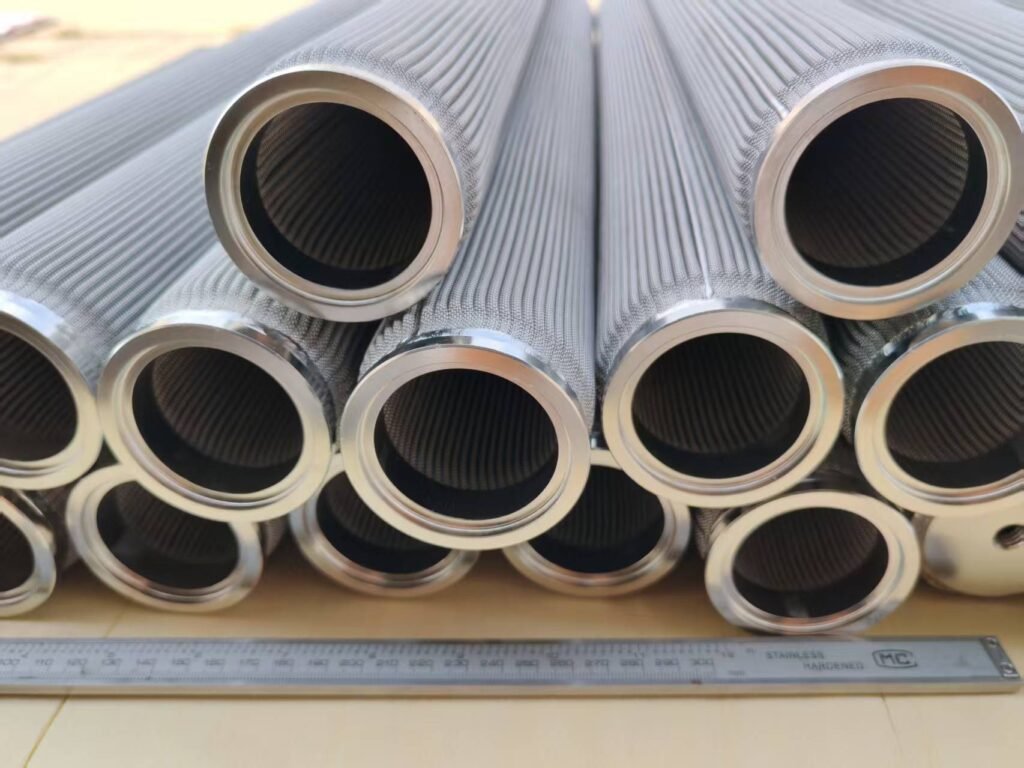
Pleating fits more medium into an envelope, but nominal medium area is not the same as uniformly accessible flow area. Pleat spacing, depth, contact between neighboring pleats, drainage layers and the flow path into the core can change resistance. A photograph can show construction features; it cannot quantify their pressure losses.
Research by Choi and colleagues examined the dependence of low-height pleated fibrous air-filter pressure loss on geometry, flow and permeability. It supports treating pleat geometry as part of the flow problem. Its fitted equations are not used here as coefficients for cylindrical metal liquid cartridges. [5]
A longer cartridge may provide more medium area, but it also changes the internal flow path and potentially the distribution along the element. Doubling nominal length therefore does not automatically halve total pressure drop. ISO 4022 itself excludes certain very long, narrow hollow test pieces where bore losses cannot be neglected relative to wall losses. A material-permeability test is not a complete assembly model. [2]
When a design changes length, pleat count, core, support or connector, identify what changed and request a corresponding curve or validated calculation. Keep the selected medium’s retention requirements alongside the clean resistance target; reducing resistance alone does not complete filter selection.
A pressure-drop estimate is not the actual system operating point
The example answers a conditional question: what pressure difference is needed across the identified assembly if its flow is 30 L/min? It does not establish that the equipment will actually deliver 30 L/min.
For a centrifugal pump at a specified speed, determining the operating point requires the pump head–flow curve and the complete system characteristic curve. [7] The system can also include piping, valves, other equipment and static head. Convert pressure and head using the relevant liquid density and a consistent basis.
Variable speed, throttling, flow control or a positive-displacement pump requires the corresponding control and supply information. A cartridge curve alone cannot determine the actual flow in every system. First evaluate resistance at the specified flow, then check the complete installation and the relevant structural limits.
Comparing clean, loaded and cleaned elements
Compare pressure drop at comparable flow, viscosity, temperature, direction and measurement boundaries. A higher reading at cold start does not, by itself, prove that the medium is more contaminated. Likewise, a lower pressure drop after cleaning does not prove restored retention, an intact seam or a sound seal.
Define the clean reference and the allowed clean pressure drop at the required flow. Define the terminal or intervention differential pressure separately, using the relevant component limits and process requirements. There is no single cleaning threshold that can be assigned to all pleated metal cartridges.
After cleaning, compare the measured curve with the appropriate reference and perform any required integrity, dimensional or retention checks. For dimensional identification before a replacement, use the replacement filter cartridge measurement guide. Matching the outside dimensions alone does not establish matching flow behavior.
Frequently asked questions
Can I calculate pressure drop from a micron rating?
No. The rating needs a defined retention basis, while resistance also depends on medium structure, thickness, area, pleats, hardware and fluid conditions. Obtain a relevant curve or validated model for the specified element.
Can I use water data for oil?
Only with a justified correction over the intended range or further test data. Use the oil properties at the relevant temperature and check whether an assembly’s non-viscous losses remain important. The interpolation calculator itself does not perform this conversion.
Does a low clean pressure drop prove good filtration?
No. It describes resistance under the stated conditions. Retention performance, sealing and structural integrity need their own acceptance evidence.
What if the requested flow is outside the measured range?
Obtain more measurements or a validated model covering that range. A straight extension of the last two points can hide changing flow behavior. Do not turn a convenient numerical result into an accepted operating point without supporting evidence.
What to request for a usable pressure-drop estimate
Provide the identified cartridge or drawing, medium, flow direction, liquid properties at temperature, minimum and maximum flow, and the required clean resistance target. Identify the housing and pressure-tap boundaries if the estimate is for the installed assembly. Keep the allowable differential pressure and cleaning conditions separate.
Then ask for a curve or calculation that states the test object, conditions, range and any correction method. That gives the estimate a defined use and makes comparisons between a prototype, replacement and production element meaningful. Our pleated metal filter page describes the related product; the measured-curve calculator supports queries once suitable data are available.
Technical references
- ISO 3968:2017 — Hydraulic fluid power, filters, evaluation of differential pressure versus flow. Hydraulic-filter test scope; the article does not claim a particular element’s compliance.
- ISO 4022:2018 — Permeable sintered metal materials, determination of fluid permeability. Applicable test-piece scope, viscous/inertial coefficients and the stated hollow-cylinder limitation.
- NIST SP 811, Chapter 8.8 — Viscosity. SI units and poise/stoke relationships.
- Outcalt, Laesecke and Brumback — Thermophysical Properties Measurements of Rocket Propellants RP-1 and RP-2, 2009. NIST-hosted original research states the dynamic/kinematic viscosity relation; its fuel-specific data are not assigned to filter service here.
- Choi et al., 2021 — Pressure drop and optimization meta-models for arbitrary low-height pleated filter shapes and flowrates. Pleated fibrous air-filter geometry research; no numerical model is transferred to the metal cartridges shown.
- Parker DF25 Duplex Filter Series — Pressure Drop Curves. Product-specific example of separate housing and element losses; its viscosity correction and limits apply within that documentation’s scope.
- KSB Centrifugal Pump Lexicon — Operating point. Pump and system characteristic curves for a centrifugal-pump operating point.
The worked numbers are invented arithmetic examples. The workflow is editorial engineering guidance, not a factory test report or a declared standard-compliant test procedure.